🗊 Презентация Parametric Linear Programming

Нажмите для полного просмотра!
Parametric Linear Programming, слайд №1 Parametric Linear Programming, слайд №2 Parametric Linear Programming, слайд №3 Parametric Linear Programming, слайд №4 Parametric Linear Programming, слайд №5 Parametric Linear Programming, слайд №6 Parametric Linear Programming, слайд №7 Parametric Linear Programming, слайд №8 Parametric Linear Programming, слайд №9 Parametric Linear Programming, слайд №10 Parametric Linear Programming, слайд №11 Parametric Linear Programming, слайд №12 Parametric Linear Programming, слайд №13

Вы можете ознакомиться и скачать презентацию на тему Parametric Linear Programming. Доклад-сообщение содержит 13 слайдов. Презентации для любого класса можно скачать бесплатно. Если материал и наш сайт презентаций Mypresentation Вам понравились – поделитесь им с друзьями с помощью социальных кнопок и добавьте в закладки в своем браузере.

Слайды и текст этой презентации


Слайд 1


Parametric Linear Programming
Описание слайда:
Parametric Linear Programming

Слайд 2


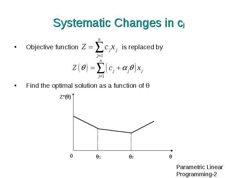
Systematic Changes in cj Objective function is replaced by Find the optimal solution as a function of θ
Описание слайда:
Systematic Changes in cj Objective function is replaced by Find the optimal solution as a function of θ

Слайд 3


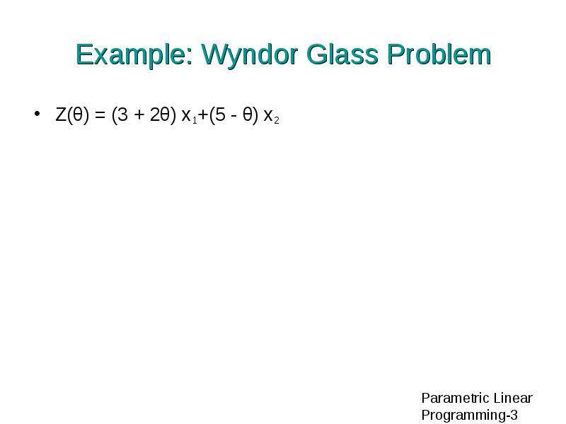
Example: Wyndor Glass Problem Z(θ) = (3 + 2θ) x1+(5 - θ) x2
Описание слайда:
Example: Wyndor Glass Problem Z(θ) = (3 + 2θ) x1+(5 - θ) x2

Слайд 4


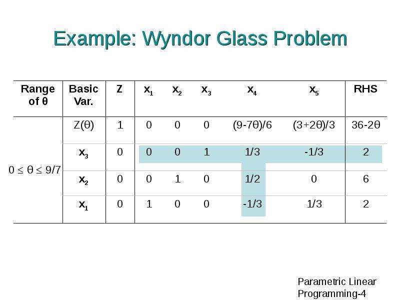
Example: Wyndor Glass Problem
Описание слайда:

Example: Wyndor Glass Problem

Слайд 5


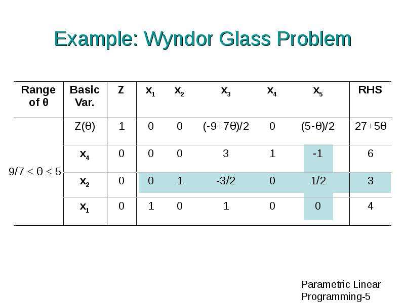
Example: Wyndor Glass Problem
Описание слайда:
Example: Wyndor Glass Problem

Слайд 6


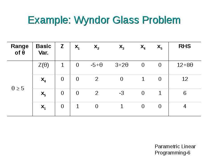
Example: Wyndor Glass Problem
Описание слайда:
Example: Wyndor Glass Problem

Слайд 7


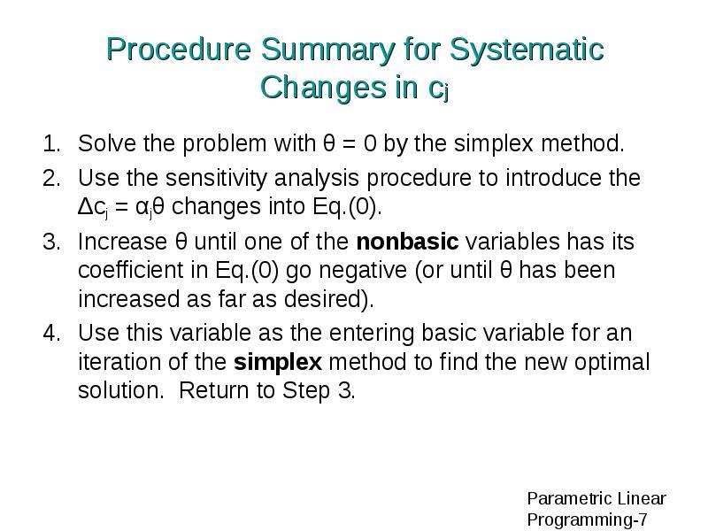
Procedure Summary for Systematic Changes in cj 1. Solve the problem with θ = 0 by the simplex method. Use the sensitivity analysis procedure to...
Описание слайда:
Procedure Summary for Systematic Changes in cj 1. Solve the problem with θ = 0 by the simplex method. Use the sensitivity analysis procedure to introduce the Δcj = αjθ changes into Eq.(0). Increase θ until one of the nonbasic variables has its coefficient in Eq.(0) go negative (or until θ has been increased as far as desired). Use this variable as the entering basic variable for an iteration of the simplex method to find the new optimal solution. Return to Step 3.

Слайд 8


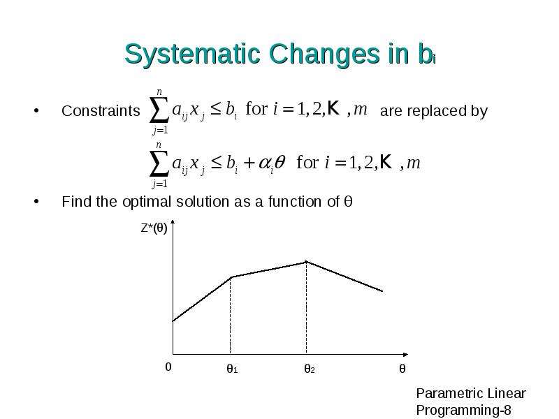
Systematic Changes in bi Constraints are replaced by Find the optimal solution as a function of θ
Описание слайда:
Systematic Changes in bi Constraints are replaced by Find the optimal solution as a function of θ

Слайд 9


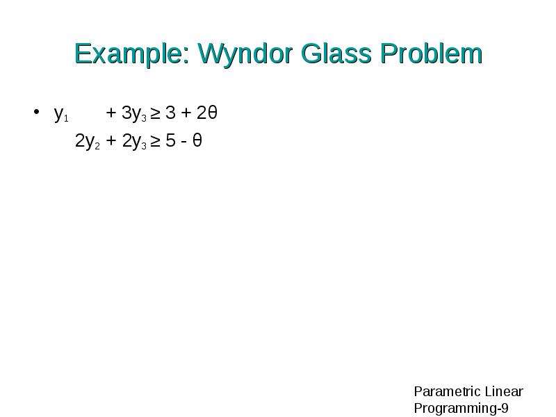
Example: Wyndor Glass Problem y1 + 3y3 ≥ 3 + 2θ 2y2 + 2y3 ≥ 5 - θ
Описание слайда:
Example: Wyndor Glass Problem y1 + 3y3 ≥ 3 + 2θ 2y2 + 2y3 ≥ 5 - θ

Слайд 10


Example: Wyndor Glass Problem
Описание слайда:
Example: Wyndor Glass Problem

Слайд 11


Example: Wyndor Glass Problem
Описание слайда:
Example: Wyndor Glass Problem

Слайд 12


Example: Wyndor Glass Problem
Описание слайда:
Example: Wyndor Glass Problem

Слайд 13


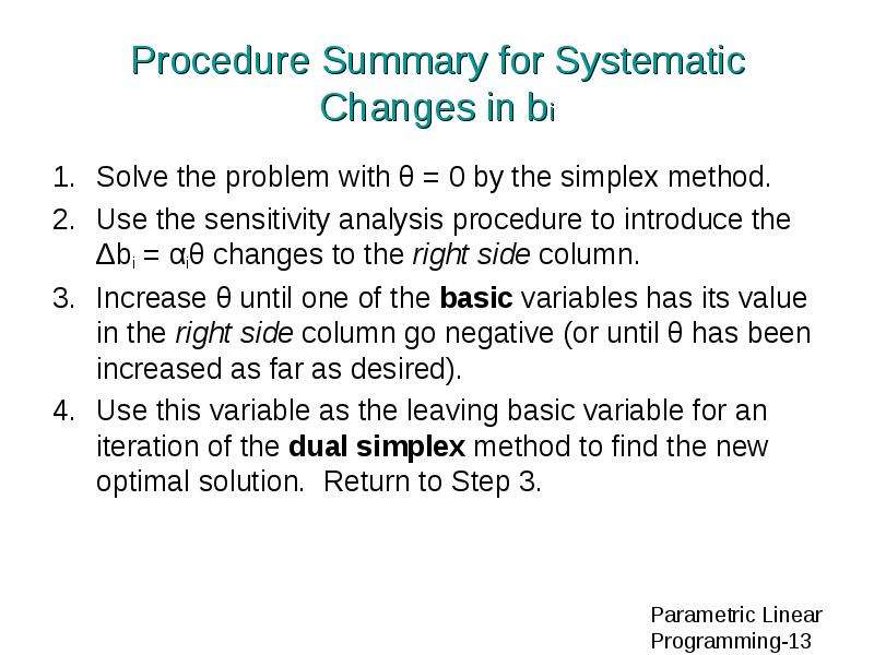
Procedure Summary for Systematic Changes in bi 1. Solve the problem with θ = 0 by the simplex method. Use the sensitivity analysis procedure to...
Описание слайда:
Procedure Summary for Systematic Changes in bi 1. Solve the problem with θ = 0 by the simplex method. Use the sensitivity analysis procedure to introduce the Δbi = αiθ changes to the right side column. Increase θ until one of the basic variables has its value in the right side column go negative (or until θ has been increased as far as desired). Use this variable as the leaving basic variable for an iteration of the dual simplex method to find the new optimal solution. Return to Step 3.


Похожие презентации
Mypresentation.ru
Загрузить презентацию